Experimental Design Lesson During Lab
Outline
Background
A solar panel consists of some number of individual solar cells packaged together for durability and practicality, and wired together to produce a single electrical output. A solar cell, also called a photovoltaic cell, produces electrical power by absorbing energy from sunlight. You can find extensive information on photovoltaics here and in many other places, but in this manual we will present the bare bones you will need to understand and carry out an original investigation.
When a photon is absorbed by the silicon material of a solar cell, the photon’s energy can excite an electron to flow freely in the material. In slightly more detail, silicon contains electrons in lower-energy states called the valence band, and there is an energy gap (bandgap) of about 1.1 eV between these states and the higher-energy, freely-moving states in the conduction band. (Recall that 1 eV = 1 electron volt = 1.6\(\times 10^{-19}\) J.) A photon with an energy above 1.1 eV can excite an electron to the conduction band and get it moving there with some kinetic energy. Electrons that simply fall back to the valence band release their energy in the form of a photon again, or in the form of lattice vibrations in the silicon; either way, no useful work is done. But when the solar panel is part of a complete circuit, excited electrons can flow out of the silicon into the external circuit and deliver some of their extra energy to a device or load in that circuit before returning to the solar cell and filling an available spot (called a hole) in the valence band again.
How do we characterize the electrical power, or energy per unit time, that we can extract from a solar panel? Here some basic circuit vocabulary will be useful. A solar panel is used as the power source for a complete circuit, or loop, in which electrons can flow from the source through the load and then back to the source, as sketched in the figure below:

Above we see a simple electrical circuit on the right, with a resistor of resistance \(R\) acting as the load. On the left is a sketch of a more tangible analogy: a water circuit in which a pump pushes water around a loop where the water gives up energy getting through an obstruction before returning to be pumped again.
Each electron flowing through the load delivers a certain amount of energy there. One way to calculate the power \(P\) delivered to the load is therefore: \begin{equation} P = \frac{\text{energy delivered to load}}{\text{time}} = \Bigl(\frac{\text{num. electrons}}{\text{time}}\Bigr)\Bigl(\frac{\text{energy delivered}}{\text{electron}}\Bigr). \end{equation}
The amount of electrical charge flowing past a point in a circuit per unit time is called current, and traditionally denoted by the variable \(I\). Likewise, the energy change per electrical charge between two points in a circuit – in this case, before and after the load – is called voltage, and traditionally denoted by the variable \(V\). Thus a rephrasing and generalization of Eq. 1 is: \begin{equation} P = I\times V. \end{equation}
It takes many, many electrons per second to generate a useful electrical current. Instead of recording currents in units of electrons per unit time, we measure in standard units of amperes or amps (A): \(1 \text{ A} = 1 \frac{\text{coulomb}}{\text{second}}\), and the charge of an electron is (negative) \(1.6\times 10^{-19}\) Coulombs. And instead of measuring voltage in units of energy given up per electron, we measure in standard units of volts (V): \(1 \text{V} = 1\frac{\text{joule}}{\text{coulomb}}\). If current in Amps is multiplied by voltage in Volts, the result for power comes out in joules per second, or watts (W).
In the electrical circuit above, the load is characterized by its electrical resistance, denoted by the variable \(R\) and measured in standard units of ohms (\(\Omega\)). The resistance of the load connected to a solar panel influences the panel’s output power through both the current and the voltage. A small load resistance means that the load does little to obstruct the flow of electrons, so in this situation current will be large, up to the maximum imposed by the fact that photons are only exciting electrons in the solar panel at a certain rate. However, if electrons don’t need to do much work to get through the small load resistance, they will deposit very little energy in the load, meaning that the voltage will go to zero as the load resistance goes to zero. Conversely, a large load resistance will restrict the flow of electrons and make \(I\) tend toward zero, but \(V\) will be larger – up to a maximum imposed by the fact that electrons are only leaving the solar panel with a certain amount of energy available for them to deposit in the load.
In evaluating the performance of a solar panel connected to a load resistance, there are three quantities of particular interest. One is the maximum current referred to above, produced when the load resistance is very small. A small or zero load resistance is called a short circuit, so the maximum current output of a solar panel is called its short-circuit current, or \(I_{\rm sc}\). The second quantity of interest is the maximum voltage output discussed above, produced when the load resistance is very large. A large or infinite load resistance is called an open circuit, so the maximum voltage output of a solar panel is called its open-circuit voltage, or \(V_{\rm oc}\). Finally, the quantity that is probably most important in the end is the panel’s maximum power output, \(P_{\rm max}\), which must be found by mapping out the values of \(I\) and \(V\) (and thus \(P\)) for different values of \(R\).
Really, all three quantities of interest can be found by varying the load resistance and measuring \((V, I)\) at each value of \(R\). A graph of \(I\) vs. \(V\), known as an I-V curve, should show something like the following: current decreasing as voltage increases, which happens as the load resistance is increased; current approaching \(I_{\rm sc}\) as \(V\) approaches zero; voltage approaching \(V_{\rm oc}\) as \(I\) approaches zero; and a “corner” in the graph between the horizontal and vertical asymptotes, where the power is maximized. A solar cell performing well shows these features clearly on its I-V curve, while one whose performance is compromised might have a distorted curve shape. You will be measuring I-V curves for your solar panel under different conditions during this lesson.
Goals for This Week
Your goals for today are to become familiar with a solar panel circuit and the data-taking process, characterize the solar panel’s performance under good lighting conditions, and get ideas for what kind of systematic investigation could be interesting and informative if you choose this experiment for your Tech Report.
First you will set up a circuit to connect your solar panel to a variable load resistance, while including multimeters to measure the current through the load and voltage across the load. You will collect data by varying load resistance and plot an I-V curve for your panel when it is fully illuminated by the grow light at your station. You will determine \(I_{\rm sc}\), \(V_{\rm oc}\), and \(P_{\rm max}\) from your data. This process will give you an idea of how to efficiently collect the relevant data, as well as what factors cause the most uncertainty in your determination of the three key quantities.
Next, you will vary the lighting conditions in some (single) way, and characterize the performance of your solar panel under the new conditions. You will share results with the rest of your class, and from there begin to think about how you might design a systematic investigation using this apparatus, in case you choose it for your Tech Report.
Instrumentation
Using cables available at your station, connect your solar panel to a variable load along with an ammeter to measure current and a voltmeter to measure voltage. The circuit you should create is shown schematically below, but we will also go one-by-one through the circuit symbols and the actual pieces of equipment they represent.
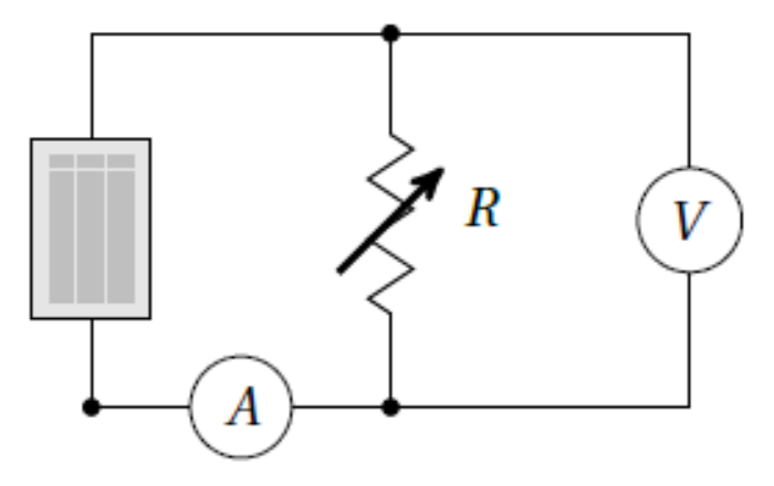
The figure above shows the circuit schematic for measuring the \(I-V\) curve of a solar panel, shown as a gray rectangle. A variable resistor provides the load, a voltmeter measures the voltage across the load, and an ammeter measures the current flowing through the load.
To operate your panel, slide the solar panel into the gap at the bottom of the black plastic light box, with solar cells facing up, and turn on the grow light in the top of the box:
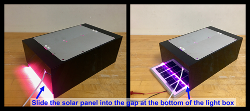
In the image on the right above, the solar panel still needs to be pushed a few more inches so that it fits entirely within the light box. The grow light provides a standardized source of illumination, and the black box isolates the panel from variations in external room lighting.
By convention red and black denote places current will flow from and to, respectively, so you should connect the red lead of the solar panel output to the load resistor, following the circuit schematic at the beginning of this section.
A load with variable resistance will be provided by a decade resistance box, shown in the figure below:
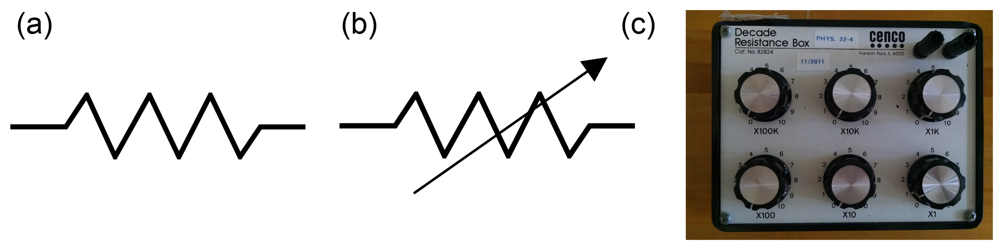
Part (a) above shows the circuit schematic symbol for a resistor. Part (b) shows the symbol for a variable resistor, and part (c) shows the actual resistor box you will use in the lab. You may have learned in the past that it is dangerous to connect a circuit with a load resistance of zero. This is true for many power sources, which may try – and fail – to produce infinite current when presented with zero resistance. Because our solar panels have another factor (number of photons absorbed per second) limiting their maximum current output, it is not dangerous to set the load resistance to zero in this particular circuit.
For the voltmeter and ammeter in your circuit, you will use two different digital multimeters, instruments that can be set to measure a variety of electrical properties of a circuit or individual device.
To measure current, you will use the desktop multimeter pictured below:
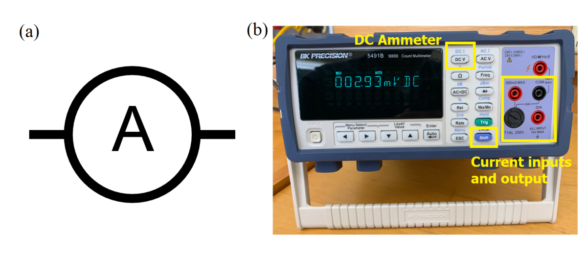
Part (a) above shows the circuit schematic symbol for an ammeter, while part (b) shows the instrument you will use. Power on the multimeter and press the “Shift” and “DC V” buttons to set it to measure DC current (see blue “DC I” above the “DC V” button). There are two red current ports labeled with the max amount of current they can measure: 500 mA and 20 A. It is generally good practice to start out using the 20A (higher-current) port if you do not know what current to expect. However, if you observe currents consistently below 500 mA or even what looks like zero current (i.e., too small to read on the 20A setting), switch to the 500 mA port for greater sensitivity. Current coming from the load should be connected to the appropriate red current input of the ammeter. Current will then flow through the ammeter and out the black COM port, which should be connected to the black lead of the solar panel to complete your circuit.
This is a good time to set up your circuit with the solar panel, load, and ammeter all in a single loop (in series with each other) so current flows through each in turn. Make sure the ammeter is reading a current (in units of A or mA).
The last component you will add is your voltmeter. For this purpose you will use a handheld multimeter like the one pictured below:
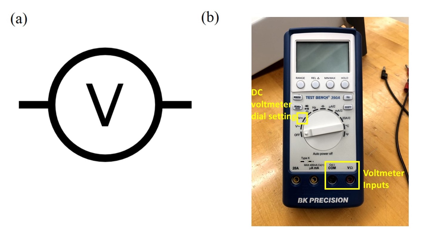
Part (a) above shows the circuit schematic symbol for a voltmeter, while part (b) shows the instrument you will use. Power on the voltmeter by turning the dial to measure DC voltage, as indicated in the picture. Since voltage is the energy change per unit charge in going from one point in a circuit to another, a voltmeter must be connected to two different points on the outside of an already complete circuit loop. This is called connecting it in parallel with the rest of the circuit. You will connect your voltmeter leads to the two sides of your load as shown below:
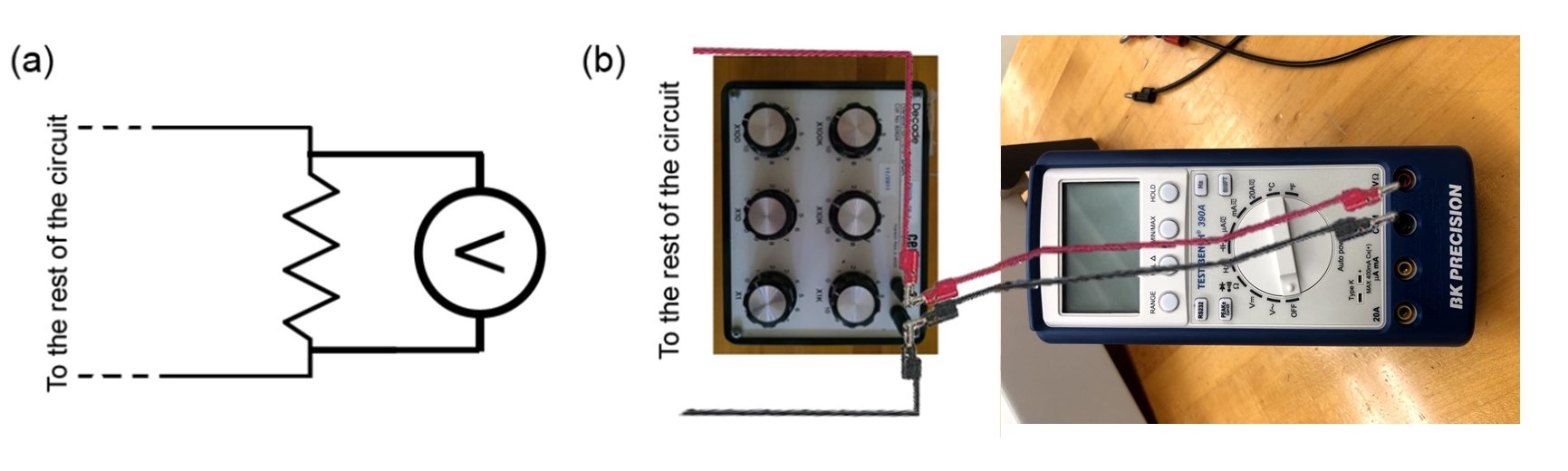
Make sure your voltmeter is reading a voltage (in units of V or mV). Be aware that either of your meters may autoscale as the current and voltage values change; make sure to pay attention to the units on the displays so that you are recording current and voltage accurately. After it has been powered on for a long time, the voltmeter might beep and possibly turn itself off, but you can always just turn the dial to off and then back to DC volts.
Data Collection
With your circuit complete, both meters powered on and set correctly, and your grow light fully illuminating your solar panel, now you will measure the I-V curve of your solar panel. To measure the I-V curve, vary the load resistance and record current and voltage values at different load resistances \(R\). To make the best use of your time, you may want to start by increasing or decreasing your load resistance by a factor of ten at a time, until you have an idea of roughly what resistance is “very large” for this solar panel – i.e., large enough to make the current start nosediving toward zero. You can then take a modest number of data points at “very large” and “very small” resistance values, but focus on intermediate resistances in order to find \(P_{\rm max}\).
To help guide your data taking, set up your Google Sheet to make a scatter plot of \(I\) vs. \(V\) values as you enter data. A second scatter plot of \(P\) vs. \(R\) can also be useful for finding \(P_{\rm max}\) efficiently. For instructions on how to make the scatter plots, see here and here, or talk to a classmate or instructor.
Your data collection for this fully-illuminated solar panel should be complete by the end of the first hour of lab. After that, you will move on to an exploration of what happens when part of the solar panel is shaded, or the light illuminating it is dimmed. We have provided you with black cardboard, scissors, and tape. Use them to cover portions of your solar panel and/or grow light, and record what you have done using the template images in your lab notebook Google Doc. Start small, and avoid covering entire cells of the panel. The cells in the panel are wired together, so the power output drops off steeply when even a few cells are covered: a previous Physics 50 student found that covering just two of the panel’s 36 cells cut \(P_{\rm max}\) in half, and covering four cut it by 80%. You will get a more meaningful comparison by covering part of a single cell, or by dimming the grow light, than by covering large areas of the panel. Repeat your data collection to find an I-V curve and key performance metrics for this new lighting situation.
At the end of lab today, all lab groups will share their explorations and results with each other. As you consider your own results and those of your classmates, think about what systematic investigation you might design using this apparatus, in case you choose it for your Tech Report. In such a systematic investigation, you would adjust some feature of the lighting/shading situation for your solar panel while holding other factors constant, to study how your solar panel’s performance – characterized by \(I_{sc}\), \(V_{oc}\), or \(P_{max}\) – varies as a function of the quantity you changed.