Physics 50
Module 3
Harvey Mudd College
Week 4: Finalizing and Communicating Results
Please note that you have two weeks to prepare your deliverable. Remaining deadlines are as follows:
- Week 4 mini-questions: due Thursday, April 29 (1pm)
- Module 3 deliverable: due Thursday, May 6 (1pm)
This week we will take another look at your analysis leading to the estimated wavelength of your laser and provide advice for communicating your results through a sequence of figures.
Experimental Iteration
We noticed that many of your results showed significant discrepancies between the results measured with the two gratings. Please take a moment to reflect on those results. As a scientist, you must often track down the source of seemingly contradictory results: was the experiment flawed, or does the theory need to be modified?
Did your results from the two differently spaced diffraction gratings agree? Did they agree with the wavelength specified by the manufacturer?
By now you should have given serious consideration to possible sources of experimental error. Here are a few of examples:
-
We provided five diffraction gratings for each diffraction grating spacing. In week 1 did you look at the x values for several gratings? Did you either find the difference to be negligible or randomize across gratings in weeks 2 & 3?
-
Were you careful to ensure your beam path was perpendicular to the screen? It can be helpful to compare the distance to the first maxima to the left and right as part of this consideration.
-
Were you careful to ensure your beam path is horizontal?
-
Did you collect data over a wide range of L values?
-
What other sources of error can you think of?
Most students should not need to collect any new data this week. If no concerns were raised with your checkpoint and you feel you already made an effort to control these potential sources of systematic error you can proceed straight to the mini-question. However, if issues were raised with your checkpoints we encourage you to check in with us in office hours.
Miniquestion 1: What next?
Click here to open in a new tab
Please do not read further until you have answered the above mini-question
In the background theory of week 1, we made a geometric argument to determine the location of interference maxima for a two slit diffraction pattern:
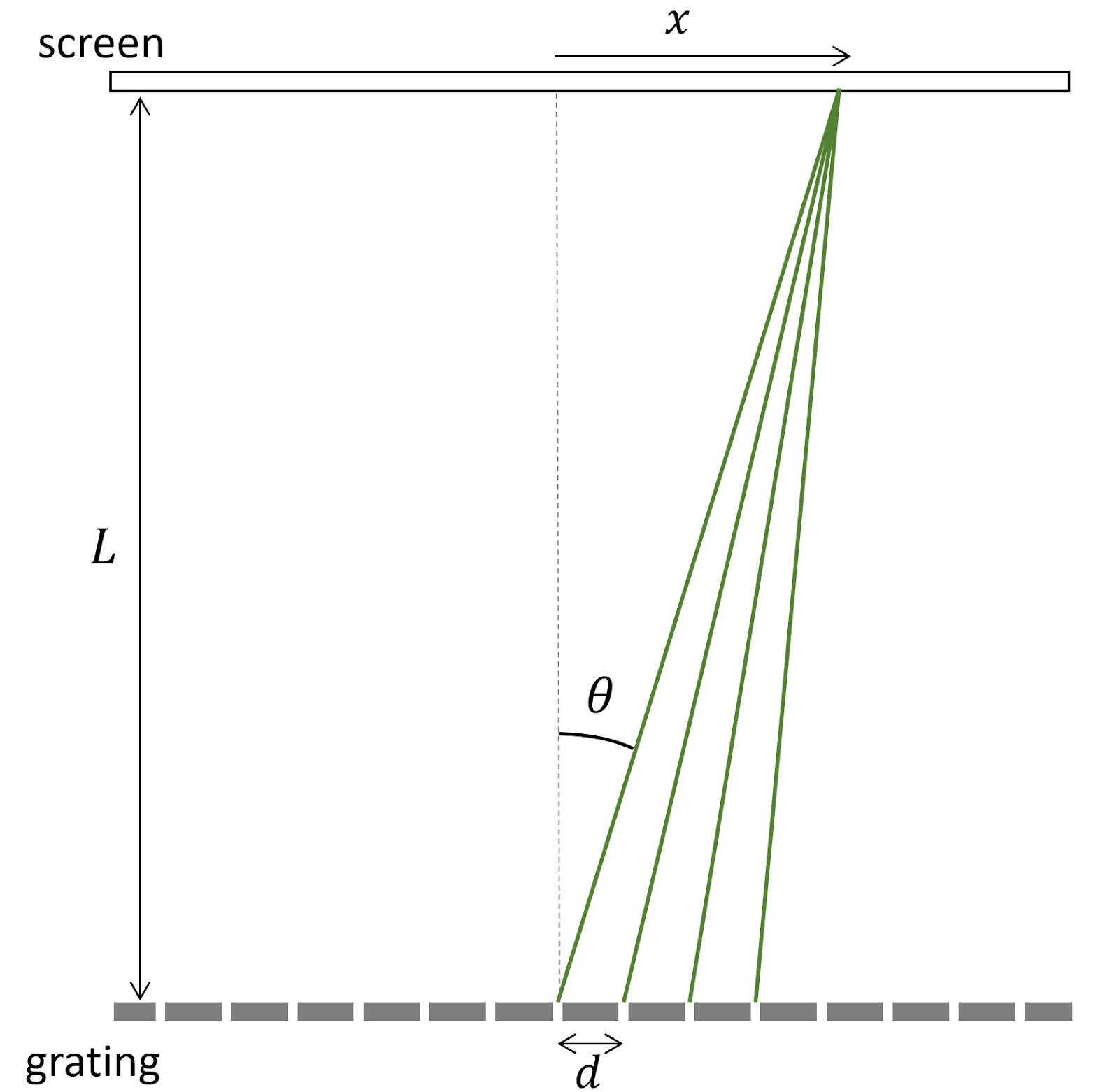
and argued that when the extra distance \(d \sin \theta\) traveled by light on adjacent rays is equal to an integer number of wavelengths, then all the rays will interfere constructively at the point where they land on the screen, creating a bright spot.
Mathematically, this condition is met if \(d \sin \theta = n \lambda\), where \(n\) is a positive integer and \(\lambda\) is the wavelength of the light.
From the figure above, we determined that \(\sin \theta = x / \sqrt{(x^2 + L^2)}\), and then made the approximation that \(x << L\) so we could approximate that \(\sin \theta = x / L\). We then substituted this into our constructive interference condition to give:
\begin{equation}\label{eq:sYoung} \frac{xd}{L} = n \lambda \end{equation}
But if we hadn’t made that approximation, we get
\[\frac{n \lambda}{d} = \frac{x}{\sqrt{x^2+L^2}}.\]Setting \(n=1\) for the first diffraction maximum and dividing the numerator and denominator on the right hand side by \(L\) gives,
\[\lambda = d \frac{x/L}{\sqrt{(x/L)^2 + 1}}.\]Then using the slope, \(m\), of our \(x\) vs. \(L\) linear regression, with \(m=x/L\), we arrive at our main result: \begin{equation} \label{eq:Young} \lambda = d \frac{m}{\sqrt{m^2 + 1}} \end{equation}
This week we will recalculate our measured value of \(\lambda\) from the correct version of Young’s equation (Eq.\eqref{eq:Young}). The good news is that we don’t have to collect any more data! The slopes we measured from the \(x\) vs. \(L\) plots of our data are not affected by the theory, so we only need to recalculate the measured wavelength based on data we have already collected.
To get a sense of how significantly this would impact our different diffraction gratings, we can rearrange Eq.\eqref{eq:Young}
\[m = \frac{\lambda/d}{\sqrt{1-(\lambda/d)^2}},\]which shows that the correct version of the theory introduces an extra factor of \(\sqrt{1-(\lambda/d)^2}\). According to this analysis, please answer the miniquestions below.
Miniquestion 2: How does the correction in Young’s formula compare for the two diffraction gratings?
Click here to open in a new tab
Miniquestion 3: Which grating will require a more significant correction?
Click here to open in a new tab
With the correct version of Young’s equation in mind, please go back and recalculate your wavelength with uncertainty for your data. You will need to propagate the uncertainty using the techniques we have used for Module 1 and Module 2. If you’d like a refresher, please review the Propagation of Uncertainties lesson from Module 1. To make sure that you have done the uncertainty propagation correctly, please answer the miniquestion below.
Miniquestion 4: Wavelength uncertainty
Click here to open in a new tab
Week 4 tasks
You have two tasks this week:
-
Redo your analysis with the corrected theory. You should be able to accomplish this by just changing a few formulae in your spreadsheet (note that both the formula for the wavelength and its uncertainty will require correction. You will need to use the calculus-based method of the previous modules to propagate the uncertainty from the slope of the x v.s. L plot to determine the uncertainty in wavelength with the revised theory (see mini-question 4). This does not require collecting any new data. Once you have recalculated the wavelength with uncertainty for the two differently spaced diffraction gratings you should regenerate the plot of wavelength v.s. diffraction grating spacing from last week and fit a horizontal line as we did in module 2 to generate your estimated wavelength with uncertainty from the plot.
-
Your second task is to prepare a sequence of 2 figures with captions to submit for your deliverable. These figures will come directly from the work you have done in the preceeding 3 weeks.
Formatting tips
-
The legends generated by the MATLAB curve fitting script introduce some possibly unimportant information for your reader. You can place a white box in Powerpoint over top of the plot legends, and then put the relevant information in the figure caption.
-
Getting the right font size and aspect ratios of your plots can be tricky. Check out this hack from Prof. Gerbode:
Deliverable – Sequence of Figures
Your module 3 deliverable will consist of 2 figures. Each of these figures must include a caption following the guidelines provided for modules 1 and 2. We encourage you to refer back to the figure preparation guide from module 1. Note that if the perspective of your picture of your experimental set-up makes it difficult to accurately define a reasonable scale bar (i.e. the length would be different at different depths of the picture), you can as an alternative use something in the picture to provide a length scale. For example, if the caption indicates the length of the laser or the spacing of the grid marks this would be sufficient to convey the length scale to the reader. The following should be submitted on Gradescope:
-
Practice calculation: the practice calculation on Gradescope will ask you to calculate the wavelength and propagated uncertainty for sample data.
-
Figure 1: Figure 1 is equivalent to the figure you submittedfor week 1, but with a caption. If any issues were raised with your week 1 checkpoint we encourage you to speak to us and make appropriate corrections before submitting your deliverable. Since resetting parameters such as the position/angle of the diffraction grating were an important part of the experimental procedure for this experiment, this should be mentioned in your caption as part of the experimental procedure.
-
Figure 2: Figure 2 will also be a multi-panel figure. -Panel (a) will showcase how you determined the wavelength. Namely, panel (a): Provide a single example plot of x v.s. L for one of the diffraction grating spacings (just as we only provided one example plot for how the terminal velocity was determined in module 2). This plot can come directly from one of your previous checkpoints figures. -Panel (b): plot of wavelength v.s. diffraction grating spacing. For this plot you should make use of the revised theory to calculate your wavelength and uncertainty from your results for the two grating spacings. Your plot should include a horizontal line fit to the two data points as well as dashed horizontal lines indicating the uncertainty of the fit (analogous to the plot you were asked to prepare for the module 2 deliverable). Your caption should include your primary result (estimated wavelength quoted with uncertainty using appropriate significant figures).
Please note that you will need to upload each figure three times.
Mini-questions:
And to double-check, make sure you have finished all of this week’s mini-questions by checking here