Week 3

1. Data Collection
2. Background on LCD Screens
3. Diffraction from an LCD
4. Week 3 Summary of Data to be Collected
5. Checkpoint 3
6. Mini-questions

This week you will continue your investigation of the wavelength of your laser. We would like you to follow an identical procedure to last week. However, instead of using the 500 line/mm grating you should now collect data with the 1000 line/mm grating. Take a moment to reflect on expectations before diving into the experiment. How will the diffraction pattern change when the grating frequency is 1000 lines/mm (grating period is 0.001 mm/line)?

Mini-question 1: Comparing diffraction patterns from gratings with different periods

Click here to open in a new tab

Data collection

Collect a set of data analogous to the data you collected last week but now using the 1000 line/mm grating. This will give you the necessary data to complete this week’s checkpoint. You should expect to spend the majority of your time in lab this week on this data collection and analysis.

As a reminder (repeat of last week’s instructions):

To collect a complete \(x\) vs. \(L\) dataset, make sure to do the following:

• Choose five values of \(L\). Last week we recommended a range of \(L\) values from about 15 cm to about 60 cm. You may find this more difficult when working with the 1000 line/mm gratings as the \(x\) values will be larger. You should still choose five \(L\) values over as wide a range as you can in the space you have available. Don’t be afraid to make small adjustments to the experimental setup to help you get high-quality data for a large range of \(L\) values.

• Collect five measurements of \(x\) for each \(L\) value, making sure that between each measurement of \(x\) you reset all the parameters you determined you needed to in Mini-question 3 from Week 1. Be sure to only use the 1000 line/mm diffraction grating. You should enter your data in the tab: “Week 3: 1000 lines/mm” in the Google sheets spreadsheet assigned to you for this class.

• For each \(L\) value, compute the mean value of \(x\) from your five trials and the random uncertainty as measured by the SEM.

• Prepare a .csv file with your \(x\pm \delta x\) and \(L\) data. There is a new tab in your Google Sheets worksheet, prepared for this: “Week 3: Plotting 1000 lines/mm data”. Be sure to change the column headings to reflect your data as these will appear as axes labels on your fit.

• Load the .csv file with your data into the curve fitting script introduced previously, selecting “linear” under the “kind” pull-down menu.

• You should make use of your data, the best fit analysis and the provided theory to determine the wavelength of your laser. You will need to use the methods you have been taught in previous modules to propagate uncertainty and determine the uncertainty in your final result.

---

Comparison of results from 500 line/mm and 1000 line/mm gratings

After you have collected and analyzed your data for the 1000 line/mm grating we would like you to compare these results with the results you obtained last week using the 500 line/mm grating. You will be asked to answer a question about your results on the checkpoint.

---

Background on LCD screens

How does what we’ve learned in this module apply to an LCD screen? We can think of a liquid crystal display, or LCD, as being a two-dimensional diffraction grating.

To get a sense of what the diffraction pattern of a two-dimensional grating would look like, mount a 500 line/mm grating on the optical rail as usual, so the grating lines are vertical. Hold a second grating, rotated so the grating lines are horizontal, just after it, and shine the laser through both gratings. You do not need to collect any data; just describe in your lab notebook what the diffraction pattern from a 2-dimensional grid looks like.

A liquid crystal display consists of a two-dimensional grid of small boxes called pixels (originally short for picture elements) that, together, display an image on a screen. These pixels are themselves composed of three ‘sub-pixels’ with colors red, green, and blue. If you look at your computer screen through a camera, you might be able to see the pixelated nature of the screen. Some common arrangements of pixels and sub-pixels in different devices are shown in the figure below. Voltages are applied across a pixel to control the colors and their relative intensities in that pixel.

Figure 1 — LCD sub-pixel layouts for various types of screens.

You can think of the screen as a grid of windows with either red, green or blue glass, illuminated by a bright light from behind. Some mechanism – perhaps a person adjusting the window shade – determines how much light passes through each individual window. If you stand far enough away, an adjacent set of red, green, and blue windows is too small for you to see each color separately; instead you see a splotch of color made up of whatever red, green, and blue light is getting through that set of windows. Again, if you stand far enough away, the individual splotches blend together and you see a color picture made up of dots the size of each individual window. Your computer screen, and any LCD screen –such as the one on your phone– for that matter, operate in a similar way, only the “windows” or pixels are on the order of tens to hundreds of micrometers wide. The more pixels a screen has per unit area, the greater the resolution of the screen, since there is more room for ‘perfecting’ the image on small scales.

Thus, you can think of the LCD as a two-dimensional grid of slits, where the distance between center of the ‘slits’ is the center-to-center pixel spacing, and is closely related to the resolution of the LCD screen.

When a laser beam strikes an LCD screen, the beam diffracts. If we set up a screen to observe the laser light reflected from the LCD screen, we observe a rectangular grid of bright dots, with roughly uniform spacing between maxima. By measuring the distance between these maxima and using the laser wavelength (determined in lab last week), you can determine the distance between the pixels, and thus deduce the resolution of the screen, by employing the same equation you used to determine the wavelength of your laser with the diffraction gratings.

In Lab Instructions for Diffraction from an LCD

Each station should have an LCD panel in an acrylic case that is fastened to an optical post and mounted on the optical rail, as shown in the figure below.

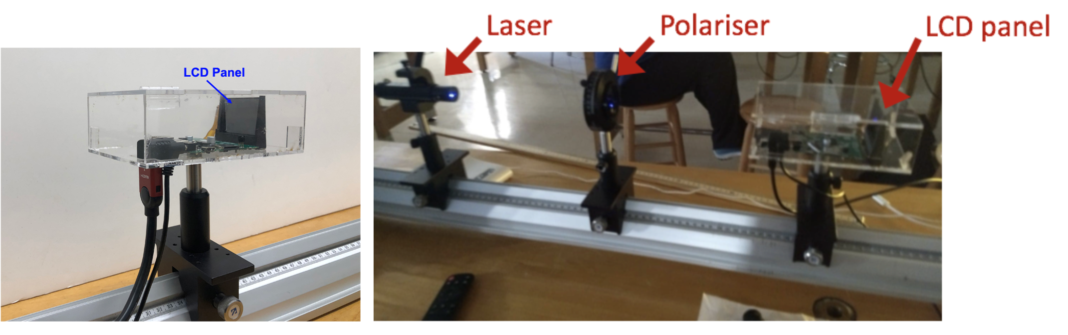
Figure 2 — (left) The laser beam should travel from left to right through the LCD panel. (right) Layout of components on the optical rail. Click on the image to see a larger version.

The HDMI cable to connect the LCD display to a computer, as well as the power cable, are attached to the LCD panel. You will not need to use these cables at all for this simple investigation. Please do not attempt to unplug either of these cables from the acrylic box. The LCD should be oriented so that the laser shines through it in a direction going from left to right in the figure on the left above.

Figure 3 shows a photo taken of our LCD screen via the eyepiece of a microscope. You are encouraged to observe the LCD screen under the microscope (through the eyepiece) in the rear of the lab. A microscope calibration slide is available that you can use to estimate the pixel spacing and compare with your results. You may find this helpful when assessing if your results are reasonable for the final question on the checkpoint.

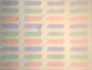
Figure 3 — Microscope image of an LCD panel identical to the one you have on your optical rail. Note: the LCD that is pre-placed in the microscope is the same model as the one on your optical rail. Please do not disassemble your own LCD or its housing, and please do not touch the LCD screen.

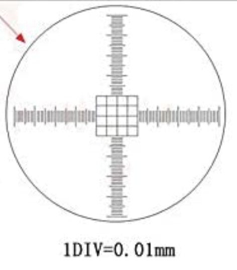Figure 4 — There is a calibration slide by the microscope that you can use to calibrate length scales in your image. The finest lines in the grid feature near the center of the slide are \(10 \mu m\)

Mount the LCD on your optical rail and shine your laser through the LCD. You will see a pattern of bright dots creating a rectangular grid, with roughly uniform spacing between maxima. Using the wavelength of the laser and by measuring the distance between these maxima, you can determine the spacing of the pixels and thus the resolution of the screen. For purposes of this investigation, you can use the laser wavelength you determined in Week 2 unless it was flagged as problematic in your Checkpoint 2 feedback. Alternately, you can use the laser wavelength you determined from this week’s data or by correcting mistakes in your Week 2 analysis.

Rather than make this a full-blown investigation, we want you simply to estimate the resolution, so you don’t need to make repeated measurements at different values of \(L\). You only need to measure the spacing of the diffraction peaks one time at a single \(L\) value and estimate the pixel spacing from there. You should take a measurement in both the horizontal and vertical directions, but you only need to take one measurement in each direction and do not need to estimate uncertainty.

Note that pixel spacing is the separation between a repeating unit. i.e. it would be for example the distance from the center of one of the red rectangles that you see to the center of the next red rectangle.

Once you’ve obtained the pixel separation distance, figure out how to infer the resolution of the LCD screen from this value. Note: you will need to measure the physical dimensions of the LCD using the unmounted one at the back of the class. Take care! These are very fragile, the yellow ribbon wire in particular. The box the LCD came in will be available at the front of class. Please make note of the manufacturer’s specification on the box so that you can compare your measured number of pixels when drawing conclusions about the reasonableness of your results in this week’s checkpoint.

Summary of Data to be Collected

In lab this week you will need to collect the following data:

• 5 measurements of \(x\) at each of 5 different \(L\) values (25 data points total), all measured with a 1000 line/mm grating.
• a single measurement of \(x\) in both the horizontal and vertical directions, each measured at a single \(L\) value, from the LCD panel. You do not need to estimate the uncertainty.
• Dimensions of the LCD screen to compute the number of pixels from the pixel spacing.
• It is also important that you take note of the laser wavelength as specified by the manufacturer. It is written on the laser itself. Similarly, you will need the manufacturer’s stated resolution of the LCD screen, stated on the box. You will want both for comparison with your experimental results.

Checkpoint 3

If you had any issues with Checkpoint 2 we recommend speaking to an instructor before completing your checkpoint this week, as it is very similar.

You should submit the following on Gradescope:

• The plot used to determine the wavelength of your laser. This plot must include the uncertainties of your data points and a line of best fit that has been determined with a weighted fit. As always, make sure to include units on your axis labels. You will be asked to upload this plot 3 times. You should upload the same plot each time. You do not need to write a caption.

• A link to your assigned spreadsheet with your experimental data and analysis.

• The slope you obtained from your plot, including the uncertainty. This is an intermediate result, so you should not round.

• The wavelength you have determined for your laser, with uncertainty from both the 500 line/mm grating (last week’s data) and 1000 line/mm grating (this week’s data). These are final results, so they should be rounded.

• A two-sentence conclusion which should answer the following question: Are your results from the two different gratings in agreement with each other and with the wavelength specified by the manufacturer (on the laser)?

• An estimate of the pixel spacing and and total number of pixels across the horizontal and vertical directions for the LCD screen. You do not need to estimate the uncertainty.

Mini-questions:

And to double-check, make sure you have finished all of this week’s mini-questions by checking here.