Module 2 Week 1 During Lab

Instrumentation

You will begin by setting up the experiment on an optical rail.

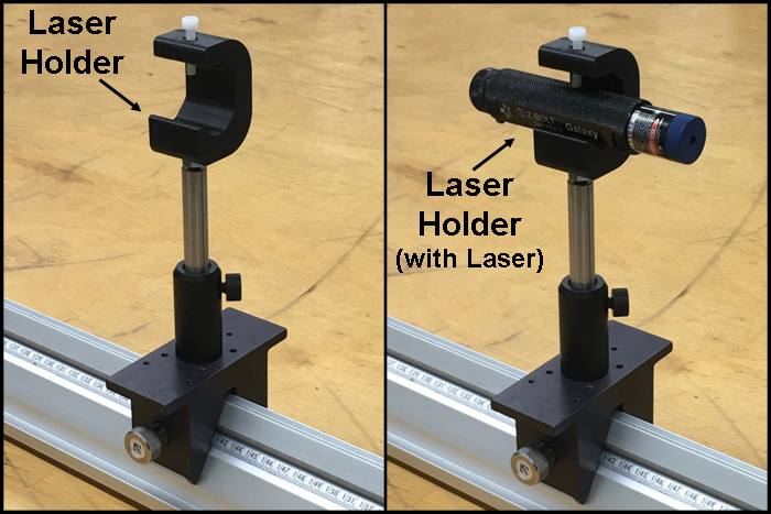
Attach the red laser to the laser holder mount, shown below in Figure 8, and attach it to a post holder placed on the optical rail with the laser facing the wall. (We don’t want the laser light shooting across the room; please make sure when you set up your laser pointer that it is aimed at the wall, away from your classmates.) When adjusting the laser, the post, or the entire mount, be sure to loosen the relevant set screw and then re-tighten it by hand once you achieve the desired positioning.

Figure 8 — Laser holder, both with and without laser itself mounted. When adjusting a piece of the apparatus, be sure to loosen the relevant set screw before making adjustments, and then re-tighten it firmly afterwards.

NEVER place your eye directly in the path of any laser beam. Even if you are sure the laser is currently off, you should never look directly down the beam path.

Mount the grid paper “screen” to the vertical support at the end of your optical rail (in the direction the laser is pointing, i.e., near the wall).

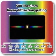
Near the center of the rail, between the laser and the screen, attach another post holder, and use it to mount a diffraction grating, shown in Fig. 9.

When handling the diffraction grating make sure to only touch the cardboard rim. Getting fingerprints on the transparent grating could affect your results and those of later lab groups.

Figure 9 — Diffraction grating. Touch only the cardboard with your fingers, and store in a vertical holder or on a piece of lint-free tissue.

Slide the diffraction grating (in its mount!) along the rail so it is very close to the screen; turn on the laser. You should see three or more dots on the screen. Slowly pull the grating away from the screen until the central three dots are spread across most of the screen. Do not pull the grating back too far, as you want to be sure that the diffracted spots are hitting the screen and not flying across the room to a neighboring lab group.

It’s possible that you will find it easier to see the diffraction patterns with the room lights turned off. After all groups have completed the basic setup of optical elements on the rail, anyone who wants to try the lights off should notify the rest of the class first. You will find a lamp at your bench that you can use to illuminate your workspace as needed.

Alternately, you may find the diffracted spots too bright; in particular, reducing the brightness of your diffraction maxima will reduce their spot size and may help with placing them more precisely later on. One way to reduce the intensity of light is by adding a rotatable polarizer. Click here for more information about polarizers. The laser emits linearly polarized light, and the polarizer will only transmit light polarized parallel to its axis, so by adding a polarizer and rotating the axis of its polarization you can control how much light gets through. Remember to turn off the laser when inserting components into the beam path of your laser. Speak to your instructor if you would like to reduce the intensity of your beam but aren’t sure how to make use of the rotatable polarizer.

The distance \(x\) between the central laser spot and the first interference maximum can be measured with a ruler or directly on the grid paper, and the distance \(L\) of the diffraction grating from the screen can be measured with a meter stick or directly from the optical rail. If you measure the position of a certain part of the grating mount instead of the grating itself, your results should come out fine as long as you are consistent (see “The Value of Plotting and Fitting” from the pre-lab).

Collecting Data

Exploratory Measurements

As in the last module, you should first perform some exploratory measurements and record them in your data sheet assigned from Google Classroom.

Please take careful note that these first measurements are just intended as a very quick exploration. We want to make sure you have time to do a careful study in the later part of today’s lab. For this first exploration please just take one quick measurement at each setting, as suggested. The settings can be approximate, and you do not need to estimate uncertainties. You are just trying to work out whether the measurement is sensitive to each parameter or not.

The ultimate goal of Module 2 is to determine the spacing of your grating by measuring \(L\) for various values of \(x\). However, at first you should get to know your apparatus and what quantities must be set carefully to give you precise and accurate results. Because this system is a little more abstract than your levitated beads, we provide a list of settings that you should be sure to check. For each setting, we ask you to change the experimental settings slightly and record how the change affects your measurements.

To get started, quickly find the \(L\) value required to produce an \(x\) value of 10 cm. Use this single trial to estimate \(d\) and check that your results are in the right range (no factors of ten or a thousand from incorrect unit conversions, for example).

Now focus on the angle of the diffraction grating, which ideally should be exactly perpendicular to the laser beam. Perhaps you might not notice if it were off by angles up to \(\pm 5^{\circ}\) (though this is actually pretty noticeable if you are paying attention). How important is this? To answer this question, first carefully set the diffraction grating perpendicular to the laser beam. You can do this by looking at the dim beam reflected by the diffraction grating. Adjust the diffraction grating so that the reflected beam retraces the incident beam (at least in the horizontal direction) by adjusting the diffraction grating until a spot from the reflected beam is visible on or just above/below the laser itself. Speak to your instructor if unclear and remember never to put your eye in the path of a laser beam. Measure \(L\) required for \(x=10\) cm under these conditions. Now purposefully “wiggle” the grating by adjusting the angle of the grating to \(\approx 5^{\circ}\) relative to the perpendicular; you can get a rough idea of the angle using a protractor held above the center of the grating. Measure \(L\) again. Now repeat the test with the grating rotated by \(\approx 5^{\circ}\) relative to the perpendicular in the other direction.

For the exploration above and those below, repeated trials are not necessary to give you a rough idea of your measurement’s sensitivity to each factor.

1. Distance from laser to diffraction grating. Change it by \(\pm\) 1 cm and record how \(L\) changes.

2. The value of the diffraction spacing \(d\) is also a parameter we can “wiggle,” in a slightly less obvious way. Each diffraction grating could have manufacturing defects that cause \(d\) to be slightly off from the stated value. We can explore this possibility by measuring \(L\) at three positions on one diffraction grating. This is just exploratory so you do not need to record the exact position you use on the grating; just take one measurement with the beam passing through the left side of the grating, one through the center and one to the right. You can adjust the position of the grating by sliding it in its holder - remember to only touch the grating by the cardboard edge. Record \(L\) for three different parts of the grating.

3. The distance \(x\) between the \(n=0\) and \(n=1\) bright spots is something we will be systematically varying later, of course. But each time we set the value of \(x\), we can only do so with some precision. Set x = 9 cm or 11 cm instead of 10 cm, and see how much the resulting \(L\) changes.

If you can think of other factors that might unintentionally influence your results, explore their effect in a similar way.

The takeaway from this exploratory exercise is that the factors that cause a larger variation in \(L\) should be carefully reset before each \(L\) measurement. The ones that don’t make much difference in \(L\) do not need to be treated with as much care.

Careful Measurements to Find \(d\)

Please go to the second sheet in your assigned Google Sheet. Week 1: Part 2 (Careful Data) which includes a template for the second half of this week’s lab.

Armed with a clear idea of which factors you need to carefully control (to reduce systematic error) and reset between trials (to randomize remaining error)… you are ready for the careful determination of \(d\) that should take the bulk of your time in lab this week.

For each of about five (no fewer) different \(x\) values, take at least five individual measurements of \(L\) and find the average and SEM of your trials. Try to pick \(x\) values that cover most of the range you can measure well with your apparatus. Also, remember to reset all the factors that also have significant effects on \(L\), for each measurement. For example, you should mess up and re-achieve the desired value of \(x\) between each of the five trials, not just leave the grating in one spot and measure its position five times.

Now you have a value for \(L \pm \delta L\) at each \(x\).

Graph your data and fit a line to it using the Physics 50 fitting routine. Use the fit results to evaluate the quality of your data set. If you are satisfied with it, calculate a final result for \(d\pm \delta d\) based on the slope of the best-fit line and its uncertainty.