Error Propagation
Functions of a Single Measured Quantity
In the uncertainty introduction, we discussed methods for finding the uncertainty for a direct measurement. Often, however, we must do some calculations with our raw data to arrive at the result we are actually interested in. Turning an uncertainty in a measured quantity into the uncertainty it causes in a calculated result is called error propagation. There is really only one basic formula that governs error propagation, and we will develop it right now.
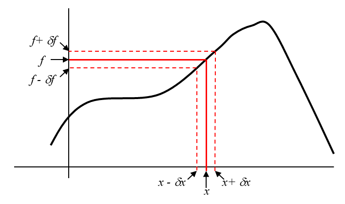
Suppose we have a quantity, \(x\), which we can measure directly with uncertainty \(\delta x\). There is a function \(f(x)\) whose value we are interested in knowing. Being uncertain about \(x\) will clearly cause some uncertainty in \(f\), so we will call this uncertainty \(\delta f\). The sketched graph below may give us some inspiration about how to calculate \(\delta f\):

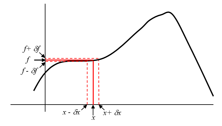
From the sketch above, it is tempting to suggest a simple rule like \(\delta f = \delta x\). But this is almost certainly flawed: what if \(f\) and \(x\) don’t even have the same units? To get a better idea of the correct relationship, consider a second sketch:

In the second sketch, \(\delta f\) is clearly much smaller than in the first sketch, even though \(\delta x\) is exactly the same in both cases. Why? Because the function \(f(x)\) is flat, or very nearly so, near the value of \(x\) we care about in the second drawing. Aha! The uncertainty in \(f\) depends on the uncertainty in \(x\), but also on the steepness of the function \(f\) in the spot where we are evaluating it. We can express “the steepness of the function \(f\)” in more precise and mathematical terms – it is the function’s derivative, \(\frac{df}{dx}\). Thus we have an error propagation rule for functions of a single variable:
\begin{equation} \delta f = \delta x \Bigl\lvert\frac{df}{dx}\Bigr\rvert, \end{equation}
where the derivative \(\frac{df}{dx}\) is evaluated at the measured value of \(x\). The absolute value signs are there because error bars give the size of uncertainties, so all error bars are expressed as positive numbers.
Example 1: Perimeter of a Square
A student measures the side length \(s\) of a square and finds \(s=4.0 \pm 0.05\) cm. They calculate that the perimeter of the square is \(p=16\) cm. To find the uncertainty \(\delta p\), they let \(s=x\) and \(p=f(x)\) in Equation 1 above, and obtain
\begin{equation} \delta p = (\delta s) (4), \nonumber \end{equation}
giving in this case \(\delta p = 0.2\) cm.
Example 2: Coefficient of Static Friction
A lab group measures the maximum angle \(\theta_m\) at which a wooden ramp can be tilted away from the horizontal before a metal container on the ramp begins to slip. They find \(\theta_m = 27.0\pm 1.4\) degrees. Using mechanics they derive \(\mu_s = \tan{\theta_m}\), so they calculate \(\mu_s = 0.509525\ldots\). To find the uncertainty \(\delta \mu_s\), they let \(\theta_m = x\) and \(\mu_s = f(x)\) in Equation 1 above, and obtain
\begin{equation} \delta \mu_s = (\delta \theta_m)(\sec{\theta_m})^2. \nonumber \end{equation}
The derivative of \(\text{tan}\) is \(\text{sec}^2\) only if \(\theta_m\) is expressed in radians, so to complete the calculation above they convert \(\delta \theta_m\) to radians before plugging in numbers. They find \(\delta \mu_s = 0.030778229\ldots\). Since digits of an answer well beyond the uncertainty are misleading, not meaningful, they write their final result as \(\mu_s = 0.51 \pm 0.03\).
Functions of Several Measured Quantities
Consider a function \(g=g(x,y,z,\ldots)\). If each independent variable has its own measured value and uncertainty, the uncertainty \(\delta g\) will have independent contributions caused by \(\delta x\), by \(\delta y\), and so forth. How can we combine them to find the overall uncertainty in \(g\)?
Let the uncertainty in \(g\) caused by \(\delta x\) be called \(\delta g_1\). From Equation 1 above, we know
\begin{equation} \delta g_1 = \delta x \Bigl\lvert\frac{\partial g}{\partial x}\Bigr\rvert, \nonumber \end{equation}
where we have changed the derivative to a partial derivative since \(g\) is a function of multiple variables. The partial derivative in Equation 2 is evaluated at the measured values of \((x,y,z,\ldots)\). However, we have similar results for the uncertainty in \(g\) caused by \(\delta y\), which we can call \(\delta g_2\), and so forth.
How can we combine all these? We have already learned how to combine unrelated (independent) errors – they add in quadrature! Thus we can write:
\begin{equation} \delta g = \sqrt{\delta g_1^2 + \delta g_2^2 + \delta g_3^2 + \ldots}, \end{equation}
which in this situation becomes
\begin{equation} \delta g = \sqrt{\Bigl(\delta x \frac{\partial g}{\partial x}\Bigr)^2 + \Bigl(\delta y \frac{\partial g}{\partial y}\Bigr)^2 + \Bigl(\delta z \frac{\partial g}{\partial z}\Bigr)^2 + \ldots}. \end{equation}
Example: Area of a Rectangle
A pair of students measure a rectangle’s length to be \(\ell = 2.0 \pm 0.1\) cm and its width to be \(w = 1.2 \pm 0.1\) cm. They calculate its area to be \(A = \ell w = 2.4 \text{ cm}^2\). To find the uncertainty, they compute
\begin{equation} \delta g_1 = \delta \ell \Bigl\lvert\frac{\partial A}{\partial \ell}\Bigr\rvert = (\delta \ell)(w) = 0.12 \text{ cm}^2 \nonumber \end{equation}
and
\begin{equation} \delta g_2 = \delta w \Bigl\lvert\frac{\partial A}{\partial w}\Bigr\rvert = (\delta w)(\ell) = 0.2 \text{ cm}^2. \nonumber \end{equation}
Combining these uncertainties from two independent sources, they find
\begin{equation} \delta g = \sqrt{\bigl((\delta \ell)(w)\bigr)^2 + \bigl((\delta w)(\ell)\bigr)^2} = 0.2332 \ldots \text{ cm}^2. \end{equation}
They present their final result as \(A = 2.4 \pm 0.23 \text{ cm}^2\).
Extra practice
This extra practice is optional – it is not assigned homework, which can be found on Gradescope!
If we have a cone with radius \(r=2.4 \pm0.3\,\textrm{cm}\) and a height \(h=10.2\pm0.4\,\textrm{cm}\), what is the volume of the cone? (Hint: \(V_\mathrm{cone}=\frac{1}{3}\pi r^2 h\))
(try it first, then click to expand/collapse) Solution:
The volume of the cone is \(V_\mathrm{cone}=\frac{1}{3} \pi r^2 h= 61.49376 \textrm{cm}^3\). But what is the uncertainty?
\[\delta V_\mathrm{cone} = \sqrt{({\delta r}\frac {\partial V_{cone}}{\partial r})^2 +({\delta h}\frac {\partial V_{cone}}{\partial h})^2 }\]\(= \sqrt{({\delta r} * \frac{1}{3} 2\pi r h)^2+({\delta h} * \frac{1}{3} \pi r^2)^2}\) \(=\sqrt{(15.37344\, \mathrm{cm}^3)^2+ (2.41152\, \mathrm{cm}^3)^2}= 15.56\, \textrm{cm}^3\)
Therefore \(V_\mathrm{cone}=(61 \pm 16)\,\textrm{cm}^3\).
Bonus: Which measurement’s uncertainty was dominant in our uncertainty in the volume of the cone, \(r\) or \(h\)?
(try it first, then click to expand/collapse) Solution:
Since the uncertainty in the volume of the cone due to the uncertainty in the radius is much larger than that from the height ( \(15.5\,\textrm{cm}^3 \gg 2.41\, \textrm{cm}^3\) ) we should refine our experimental procedure to be much more careful and precise in our radius measurement since this is limiting our knowledge of the cone’s volume.